Partitioning as a Method for Allowing Closed-Form Solutions in Simulations

Abstract

In order to approximate initial value problems in simulations, numerical methods have been developed that generally fall into either the Runge-Kutta or Linear Multistep families. This post proposes a third method, in which a complex system is separated into partitions in order to enable analytical solutions of the simplified equations. Further, for some cases the error introduced by these simplifications is smaller than the error introduced in current state of the art numerical approximations, allowing for either a smaller computational load or increased accuracy compared to current methods.

This post has three sections:

Background: Numerical and Analytical Solutions
Part 1: Basic Hybrid Numerical-Analytical Simulations
Part 2: Partitioned Hybrid Numerical-Analytical Simulations

Background: Numerical and Analytical Solutions

I’m going to start with a classic example: Let’s say Sam has a bucket with a small hole the bottom which they place under a spigot. If Sam were to turn on the water it would equilibriate at some level, with higher water levels also causing water to stream out faster. But there’s a twist: let’s say every minute Sam flips a coin, turning the spigot on or off based on the result. What is the average height of the water?

To solve this problem, we might model and simulate the system, and an early choice we have to make is whether to solve analytically or numerically.

Numerical Solution

In a numerical solution, we pick a time interval (let’s say one second) and update the state of the system every interval, called a step. Every update we might calculate the rate of water flowing into the bucket, the rate of water flowing out, take the difference, and then multiply by the time interval to get how much water has accumulated in the bucket (first-order Euler’s method). Numerical solutions can easily handle differential functions, as each new state is calculated as a function of the previous state along with the rate of change of each variable.

The major drawback to numerical solutions is that they are an approximation. For small step sizes it works well: the rate flowing in or out will not change significantly during the step, so assuming it to be constant (and updating every step) gives a fairly good result. Medium step sizes may not produce accurate results, but will yield a stable system that converges to the appropriate value given enough time. At some point, a step size too large will produce an inherently unstable system that diverges.

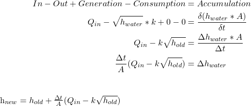
If we pretend the flowrate out of the bucket is proportional to the square root of the height of the water h, we get the following mass balance:

$\begin{align*} In - Out + Generation - Consumption & = Accumulation \\ Q_{in} - \sqrt{h_{water}}*k + 0 -0 & = \frac{\delta (h_{water}*A)}{\delta t} \\ Q_{in} - k\sqrt{h_{old}} & = \frac{\Delta h_{water} * A}{\Delta t} \\ \frac{\Delta t}{A}(Q_{in} - k\sqrt{h_{old}}) & = \Delta h_{water} \\ \end{align*} h_{new} = h_{old} + \frac{\Delta t}{A}(Q_{in} - k\sqrt{h_{old}})$

Note that $\mathrm{h_{water}}$ is given the constant value $\mathrm{h_{old}}$ for integration. Q is the volumetric flowrate, A is the cross-sectional area of the bucket, and $\mathrm{\Delta t}$ is the time since the last update.

With a means of updating the water level at each new step, we pick a constant step size (preferably a denominator of one minute) and run the simulation, averaging the step size collected at each step to gain the average step size.

Analytical Solution

An analytical solution attempts to solve the equations defining a system so that the exact amount of water at any time t can be exactly solved for. This might be done solving any given differential equation. However, analytical solutions require a closed-form expression, which only results from continuous, differentiable functions; the spigot being switched on or off would be a discontinuity.

We can borrow from Discrete Event Simulation (DES) a way of handling such events called Next-Event Time Progression. We skip to points in time where the behavior of the system changes, and only update the state at such events.

In our case, this would look like the following: the differential equations are solved with the present behavior (the spigot is either on or off), allowing for the water level to be described with a closed-form expression. Whenever the water spigot is turned on or off, the state of the system is solved for at that time, and new equations describing the system are set up that describe how the system will change with time going forward. This would be called a hybrid continuous-discrete simulation (often referred to as “hybrid simulation”), as it contains both continuous (water level) and discrete (the spigot) elements.

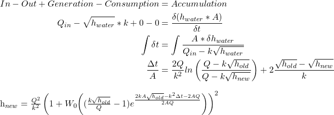
This has the benefit of being computationally cheap and exactly accurate, but requires that a closed-form expression is found. For water flowing from a bucket we have accurate models, and a chemical engineer could analytically solve the differential equation. The simulation would only have to update every time Sam turns the spigot on or off (the discrete event). Time passes instantaneously between events, and so is computationally efficient.

$\begin{align*} In - Out + Generation - Consumption & = Accumulation \\ Q_{in} - \sqrt{h_{water}}*k + 0 -0 & = \frac{\delta (h_{water}*A)}{\delta t} \\ \int \delta t & = \int \frac{A*\delta h_{water}}{Q_{in} - k\sqrt{h_{water}}} \\ \frac{\Delta t}{A} & = \frac{2Q}{k^2}ln\left( \frac{Q-k\sqrt{h_{old}}}{Q-k\sqrt{h_{new}}} \right)+2\frac{\sqrt{h_{old}}-\sqrt{h_{new}}}{k} \end{align} h_{new} = \frac{Q^2}{k^2}\left( 1+W_0{\left(}(\frac{k\sqrt{h_{old}}}{Q}-1)e^\frac{2kA\sqrt{h_{old}}-k^2 \Delta t-2AQ}{2AQ} \right) \right) ^2$

W is the Lambert W function.

Once we have solutions for the water level in each time period, we may solve for the average level in that period and use Monte-Carlo sampling (applied to the coin flips) to find the average level.

Analytical vs Numerical in Practice

While analytical solutions are preferable, the high complexity of simulations almost invariably mean that only numerical solutions are feasible for system-level simulations. There are various techniques to improve numerical solutions, including dynamic step sizes and the application of Runge-Kutta methods for better approximating a curve (think Euler’s method with higher orders). It is also common to utilize hybrid simulations, in which both discrete events and continuous variables are integrated into one simulation (this time using numerical methods instead of analytical).

Part 1: Basic Hybrid Numerical-Analytical Simulations

We would like to use analytical methods as much as possible, both for their accuracy and computational efficiency. However for CC-sim the system of equations is not solvable – both because the equations describing the system are so complex, and because there are logic functions being performed (E.G.: reaction rate may be based solely on the limiting reactant). Running it as a first-order numerical would be computationally expensive, as the step size would have to be shorter than one second just to create a stable system. A microsparger can produce $\mathrm{k_L a}$ values larger than 30 / min, and mass transfer across a cell membrane is well in excess of even that. Running a step size of one minute would be inherently unstable, as the concentration of aqueous gasses would quickly diverge (the rate of gas transfer is far faster than the simulation can handle).

The solution used by CC-sim is to divide all variables into pseudoconstant and dynamic variables in order to allow closed-form expressions to be found from solving differential equations. The “constant” variables are updated every step, and dynamic variables can be solved to the next step as in a hybrid analytical solution.

A pseudoconstant is a variable that changes with time but is treated as constant for the duration of the step. Psuedoconstants are only appropriate to be used when they will not cause stiff equation instability. Generally variables like temperature and PID outputs can be treated as constant, as they change much more slowly and do not affect the system as much as a variable like dissolved oxygen. Pseudoconstants also allow discrete events to be hidden behind a constant variable.

This is much like the simulation of Sam and the water bucket updating once a minute, and checking whether Sam turned on or off the spigot. The rate of water into the bucket is considered a constant for the interval, while the amount of water in the bucket as well as the flowrate out are dynamic variables.

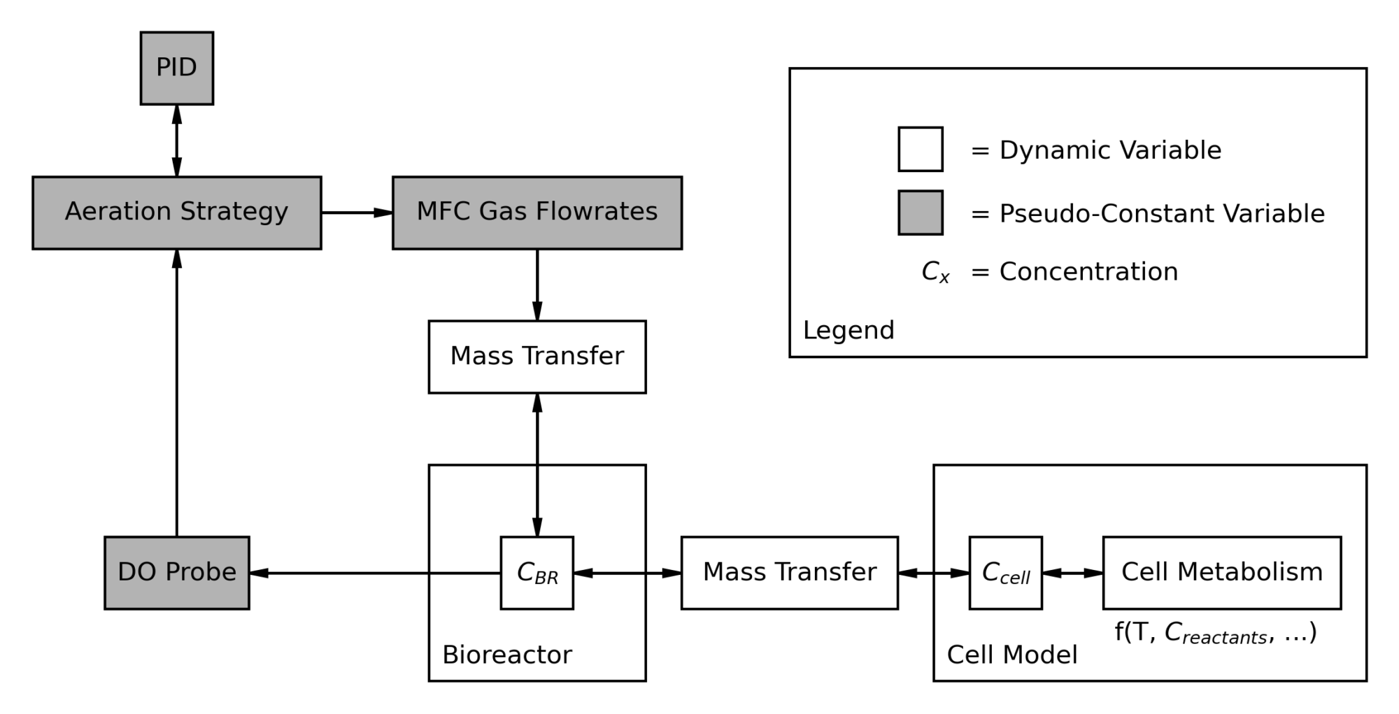
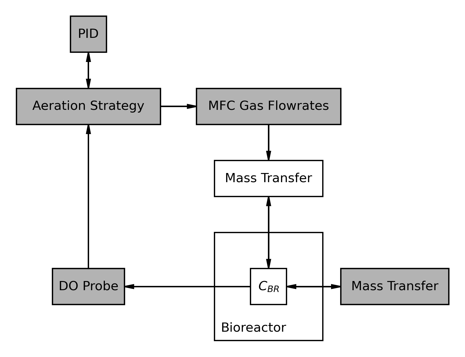
An example from CC-Sim could be the oxygenation of the cell culture followed by oxygen consumption by the cells. The full system involves the DO probe measuring oxygen levels, feeding into a PID controller, which then gets transformed into air and oxygen flowrates by the control strategy, actuation on the part of the MFC, kLa and mass transfer calculations by the environment, oxygen consumption on the part of the cells, changing dissolved oxygen concentration in the bulk fluid, and finally returning to dissolved oxygen reading by the probe.

Solving this system analytically would be an impossible task, and treating variables like mass transfer as constant would lead to simulation instability for all but excessively low step sizes. We can treat variables that do not change much over a step, such as the aeration control loop, as pseudoconstants in order to simplify the system and make it more readily analytically solvable. However, the bioreactor – cell – cell metabolism system is still not analytically solvable, so what further can we do?

Part 2: Partitioned Hybrid Numerical-Analytical Simulations

I propose a system of partitioning the system, in which a large interconnected system can be split into multiple systems by treating each other as pseudoconstants. The concentration in the bioreactor does not specifically need to know the profile of the mass transfer to cells with respect to time; an average mass transfer over the timestep would suffice. On the other hand, mass transfer to the cells needs to remain dynamic, and so the concentration in the bioreactor is instead treated as the pseudoconstant from the other side of the partition.

This image has an empty alt attribute; its file name is BR-perspective.png — Bioreactor Perspective

This image has an empty alt attribute; its file name is cell-perspective.png — Cell Perspective

The exact mechanics occur in three steps: First, the environment calculates the maximum mass transfer rate into the cells such that concentration in the environment would reach zero at the end of the step. This step is necessary to ensure concentration in the environment never goes below zero.

Second, the cell model calculates the total mass transfer into the cell, treating the environment concentration as constant, and returns an average mass transfer rate over the step for the environment. It checks that this rate does not exceed the maximum transfer rate from step one.

Lastly, the environment can solve for the accumulation of oxygen in the fluid by treating the mass transfer of oxygen into cells is constant, with concentration of oxygen in the fluid as dynamic.

When both the continuous and discrete methods are combined the system is far more stable, allowing a larger step size to be used (saving computational power) compared to a purely numerical solution with the same error.

Applications to Acausal Modeling

In acausal modeling, the user supplies a system of equations defining a system and the software figures out what the inputs and outputs are. The equations are rearranged and the order of operations determined by the software. This stands in contrast to block models, like above, in which the user must determine the order of operations and how to calculate the needed variables. Acausal modeling is a more advanced and versatile methodology that is not included in CC-Sim.

With advances in symbolic integration capabilities by computers that rival human capabilities, it should be possible for acausal modeling to incorporate hybrid numerical-analytical solutions. The missing link would be criteria for where to place the partition. While certain indicators like low rate of change would seem correlated with good partitions, it doesn’t seem to be the base reason. I suspect that it is related to concept of “stiffness” of a system, and more formal mathematics is required.

Future Work

Comparison of Errors and Computational Time by Method