Modeling Recirculation Flowrate in Bioreactors

When we model a system, there exists a tradeoff between complexity of the model and its accuracy. For example in the context of a molecule the atoms could be modeled by:

A point, with bonds connecting to other atoms
A point in space that attracts and repels other atoms – possibly with charge or a dipole
Atoms containing protons, neutrons, and electrons, each with a location and velocity (more commonly, probably just the electrons)
Same as (3), except particles have a probability density function
…increasingly complicated QD models

We generally want the simplest model that achieves our goals. If our goal were to model protein folding, we may want to stick to points with a mass and dipole that attract and repel others. If we wanted to model bond formation we would use the more complex end of the spectrum.

Modeling pumps in a simulation like CC-Sim is much the same. Level 1 might be “each pump is characterized by a volumetric flowrate”, which is sufficient when we are only talking about adding a component; most pumps in CC-Sim are modeled this way. However, when the pump deals with cells that can be sheared, control loops, pressure sensors, and sieving profiles, we need a more complicated model.

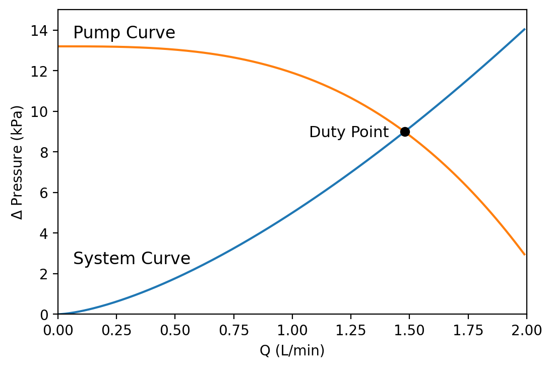
The interaction between a pump, the fluid, and the enclosure can be better understood through pressure. A pump creates fluid pressure which causes flow and dissipates as the fluid flows through the system. Since both the pressure drop through a system as well as the pressure created by a pump are functions of flowrate we can create a pressure curve, graphed as a function of flowrate, that describes the pressure created or dissipated through the component. The intersection of these two curves is the duty point – the point at which the system operates. This post focuses on creating and solving such curves in simulations such as CC-Sim along with related modeling considerations.

System Curve

The system curve plots the volumetric flowrate against the pressure drop of the system at that flowrate. It includes fluid properties along with all of the straight pipes, bends, valves, membranes, and any other part that would cause pressure loss, often resulting in a nonlinear function (especially for turbulent flow and non-Newtonian fluids).

In the case of recirculation in the context of perfusion it is easy to calculate the system curve; almost all of the pressure drop occurs in the hollow fiber, which we can use the Darcy-Weisbach equation to calculate. Our system starts with a Reynolds number of 300 and only decreases from there, so we can use the simplification $f_D = \frac{64}{Re}$ , which results in the equation $\Delta p={\frac {128 \mu LQ_{net}}{\pi n D^4}}$ . Since hollow fiber filters are composed of many fibers, I’ve used $Q_{net}$ and n to refer to the net volumetric flowrate and the number of fibers, respectively. This equation applies to Reynolds numbers of up to 2000, which holds for all perfusion regimes I have seen. It may diverge from this correlation when using fibers with large ID (>~1cm) or when fouling causes an impedance in the hollow fiber.

When thinking of flowrate and pressure drop, it can be useful to think of it in the form of $\Delta P = R * Q$ , much like resistance in an electrical circuit. The equation in the previous paragraph is particularly convenient because our resistance is constant: that is, it does not depend on the flowrate, and pressure drop and flowrate are linearly related. Depending on the shape of the pump curve, an analytical solution is possible.

Pump Curve

Unfortunately pump curves are not as well studied as pressure drop in a pipe, and we don’t have any papers providing correlations for them. With sufficient data interpolating between points is an option – although here, we’re going to fit a curve to the data instead. We’ll gather what evidence we can and create our own correlation so that we can predict performance at arbitrary pump settings and flowrates efficiently.

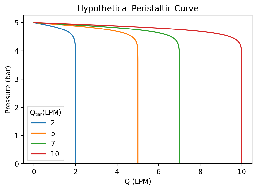
First, we note that pumps that work differently will have a different shape to their curve. Displacement pumps such as peristaltic have a mostly “inelastic” curve, in which flowrate remains more or less constant across a wide range of pressures. Pumps such as centrifugal will instead be “elastic”, and maintain a more constant pressure irrespective of flowrate. The equations describing the curve will necessarily be dependent on the type pump being used.

Centrifugal Pump Curve (from Levitronix)

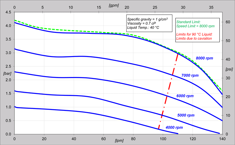
Let’s say wanted to use the Levitronix pump in our model, and had the empirical evidence seen in the graph. First, we’d need to hypothesize an equation describing the curve. I note a few things:

Pressure increases exponentially with RPM
Pressure decreases exponentially with flowrate
The decrease in pressure with flowrate is larger at higher RPM curves (and not proportional to the pressure)

Given these observations, an equation to describe the curve might have the form $\Delta P = a * RPM^b - c*Q^d*RPM^g$ , where a, b, c, d, and g are constants. In order to fit the curve, we input our data into python (preferably raw data, but here points taken from the graph):

from scipy import optimize
import numpy as np

q= np.array([0, 20, 40, 60, 80, 100, 120, 140], dtype = float)
rpm = np.array([4000, 5000, 6000, 7000, 8000], dtype = float)
data = np.array([[1, 0.9, 0.8, 0.7, 0.4, 0.2, np.nan, np.nan],
                 [1.6, 1.5, 1.4, 1.25, 1, 0.7, 0.3, 0],
                 [2.3, 2.2, 2.1, 2, 1.75, 1.45, 1.1, 0.5],
                 [3.15, 2.85, 2.8, 2.7, 2.6, 2.3, 1.8, 1],
                 [4.1, 3.8, 3.7, 3.7, 3.6, 3.25, 2.7, 1.5]],
                )

Next we scale the data; this makes it easier for algorithms to converge at the right optimal values for variables, as the scale of the data is known / uniform.

rpm_scale = rpm.max()
q_scale = q.max()
yscale = np.nanmax(data)

data /= yscale
q /= q_scale
rpm /= rpm_scale

Finally, we define our prediction function, initial values, and the cost function. Here we use scipy’s optimize module to find the ideal values for the constants.

predict_func = lambda  RPM, Q, a, b, c, d, g: a*RPM**b+c*(Q)**d*RPM**g
initial = [1, 1, 1, 1, 1]

def L2_norm(params):
  total = 0
  for RPM, curve in zip(rpm, data):
    for q_index in range(len(curve)):
      if not np.isnan(curve[q_index]):
        predicted_value = predict_func(RPM, q[q_index],*params)
        total += (predicted_value-curve[q_index])**2
  return total

result = optimize.minimize(L2_norm, initial)

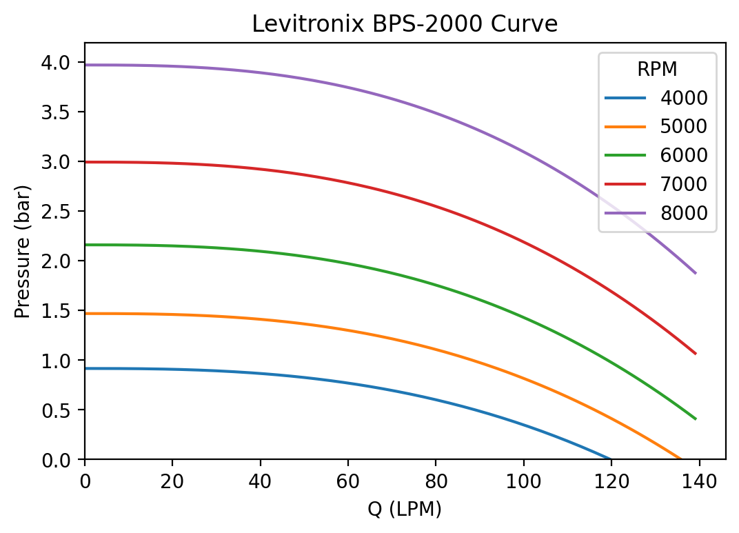
After converting to SI units and accounting for scaling, this gives us the equation $\Delta P = 1.3\mathrm{e}{-4} * RPM^{2.1} - 9.3\mathrm{e}{6}Q^{2.6}RPM^{0.6}$ . We get an RMSE of 0.029 bar across 38 datapoints, and now have enough information to find the duty point in our simulation.

[Note: Ultimately CC-Sim used this curve with an RMSE of 0.017 bar.]

Finding the Intersection

Once we have the system curve f(x) and the pump curve g(x), we need only find the root of f(x)-g(x) in order to find the intersection. This can be done with Ridder’s method or any other root-finding algorithm. Since this is a simulation and we are solving for the intersection many times we could also use the previous step’s solution as an initial guess.

If the form of f(x) and g(x) are known in advance, it may also be possible to have an analytical solution, eliminating the need for iterative methods.

Shear

As the culture ages, sieving (the amount of product making it through the filter) decreases, and so there is significant incentive to figure out the cause and find a solution to the problem. Most of what is known is that a primary factor of sieving is sheared cells, so there is an emphasis on keeping culture health high.

The reason the pump was modeled this way (as opposed to just specifying a flowrate) is because we needed to know what rate the pump is operating at, which is a function of everything from flowrate setting to liquid viscosity. The next step would be to find correlations between the pump conditions and shear created, except that shear isn’t something that is measured and I haven’t found any published correlations. Here’s what I do know:

Cells are sheared at various places in the bioreactor, with the hollow fiber and recirculation pump being the primary sources
Peristaltic pumps have a marked effect on cell shear, and low-shear pumps like Levitronix significantly increase culture health
ATF perfusion performs better in large part because the pump doesn’t shear cells – yet still suffers from decreased sieving over time
Shear increases linearly with relative speed (between two plates) and inversely with distance between the plates

As such, the best I have been able to do is program calculations that follow these observations – and hopefully, any technique that works for optimizing shear in CC-Sim could equally be applied in real experiments.

Tradeoffs and Other Considerations

There are a great number of tradeoffs to be made with the selection and fitting of the equation for the pump curve, and I’m not sure how best to select an “ideal” option. A few considerations include:

Using weights to preference normal operating range
Simpler equations with fewer number of constants (reduces overfitting)
Selecting equations that allow analytical solutions (reduced computational cost)
- Since recirculation rate is in a control loop, it won’t have much of an impact on simulation result either (and computational cost might be preferenced)
- If the fluid is non-Newtonian, we’ll have to rely on an iterative method anyway and this becomes moot

For example, when we constrain d to equal 3, we get an equation of $\Delta P = 1.1\mathrm{e}{-4} * RPM^{2.1} - 7\mathrm{e}{6}Q^{3}RPM^{0.7}$ with an RMSE of 0.03 bar that also allows for a computationally efficient closed-form expression of the duty point.

If one wanted to increase the level of detail in the model, they might also include cavitation, which would heavily shear cells. However, it can probably be assumed that an engineer is sizing the pump correctly and that cavitation does not occur; adding cavitation to the model would just waste computational power. It may be sufficient just to add a check and warning that cavitation may occur whenever the simulated pump operates above a certain range.

A more practical consideration may be non-Newtonian fluids. There is evidence that high density cell culture is shear-thinning; more accurate pressure drop can be modeled by accounting for the changing viscosity with shear rate. This would primarily affect the system curve, with lower pressure drop at higher flowrates than would otherwise be expected.

As always, if you have any thoughts, questions, or comments: feel free to comment or contact me.